# Load MASS (pre-installed in R)
library(MASS)
data(birthwt)

# Convert binary indicator variables into explicit factors
birthwt$smoke <- factor(birthwt$smoke, labels = c("Non-Smoker", "Smoker"))
birthwt$ht    <- factor(birthwt$ht, labels = c("No", "Yes"))
birthwt$ui <- factor(birthwt$ui, labels = c("No", "Yes"))Multivariate analysis
Regression diagnostics
Dr. Yu Cheng Hsu
Learning objectives
- Demonstrate linear regression diagnostics
- Judgement on the performance of linear regression
Terms matching
| Rachel’s slide | Ray’s slides |
|---|---|
| \(\text{SS}_\text{Total}\) | \(\text{SST}\) |
| \(\text{SS}_\text{Regression}\) | \(\text{SSR}\) |
| \(\text{SS}_\text{Residual}\) | \(\text{SSE}\) |
| \(\text{MSS}_\text{Residual}\) | \(\text{MSE}\) |
Overview of linear regression
In linear regression, our fundamental objective is to explain the variability observed in the outcome variable (\(Y\)) using one or more explanatory variables (\(X_1, X_2, \dots, X_k\)).
\[ \hat{Y}_i = b_0 + b_1 X_{1i} + b_2 X_{2i} + \dots + b_k X_{ki} \]
It is crucial to know:
- Do \(X_1, X_2, \dots, X_k\) really explain \(Y\)?
- How good is the model’s performance?
Recap
| Metric | Formula | Degrees of Freedom (\(df\)) | Conceptual Intuition |
|---|---|---|---|
| SST | \(\sum_{i=1}^n (Y_i - \bar{Y})^2\) | \(n - 1\) | Total variation in the outcome \(Y\) without using any predictors. |
| SSR | \(\sum_{i=1}^n (\hat{Y}_i - \bar{Y})^2\) | \(k\) | Variation accounted for by the regression model. |
| SSE | \(\sum_{i=1}^n (Y_i - \hat{Y}_i)^2\) \(= \sum_{i=1}^n e_i^2\) |
\(n - k - 1\) | Unexplained variation; sum of squared discrepancies between observed points and regression surface. |
Goodness-of-Fit: \(R^2\)
\(R^2\) (The coefficient of determination) quantifies the proportion of total variation in the response variable explained by the linear combination of predictors:
\[ R^2 = \frac{\text{SSR}}{\text{SST}} = 1 - \frac{\text{SSE}}{\text{SST}} \]
Interpretation Rules
- Range: In standard OLS with an intercept, \(0 \le R^2 \le 1\) (or \(0\%\) to \(100\%\)).
- Interpretation: If \(R^2 = 0.74\), exactly 74% of the variability in \(Y\) is explained by the predictors included in the model, while the remaining 26% is attributable to residual noise or omitted factors.
- Limitation: \(R^2\) is non-decreasing with respect to the addition of predictors. Adding completely unrelated random noise variables will force \(\text{SSE}\) to stay equal or decrease, artificially inflating \(R^2\).
Adjusted \(R^2\) (\(R^2_{\text{adj}}\))
The Adjusted \(R^2\) incorporates degrees of freedom to penalize excessive parameterization and prevent overfitting:
\[ \small R^2_{\text{adj}} = 1 - \left[ \frac{\text{SSE} / (n - k - 1)}{\text{SST} / (n - 1)} \right] = 1 - \left( \frac{\text{MSE}}{\text{MST}} \right) \]
Alternatively expressed via \(R^2\): \[ \small R^2_{\text{adj}} = 1 - (1 - R^2) \frac{n - 1}{n - k - 1} \]
Key Properties
- Increases only if a newly added predictor reduces \(\text{SSE}\) by a margin greater than what would be expected by pure chance.
- Can occasionally yield a negative value when model fit is negligible; in such cases, it is effectively interpreted as zero.
Pitfalls to Avoid
- Confusing \(R^2_{\text{adj}}\) with Causality: A high \(R^2\) indicates strong linear correlation, not causal direction.
- Comparing \(R^2_{\text{adj}}\) Across Different Transformations: You cannot compare the \(R^2\) of a model predicting \(Y\) directly to a model predicting \(\ln(Y)\), because \(\text{SST}\) is measured on fundamentally different scales.
- Over-reliance on \(R^2_{\text{adj}}\) Alone: Always inspect residual diagnostics (residual vs. fitted plots, Q-Q plots) to ensure linearity, normality, and homoscedasticity assumptions hold.
\(F\)-Test for Model Significance
\(F\)-Test evaluates whether the collection of predictors collectively explains a statistically significant amount of variation.
Hypotheses
- Null Hypothesis (\(H_0\)): All slope coefficients are simultaneously zero.
\[ H_0: \beta_1 = \beta_2 = \dots = \beta_k = 0 \]
- Alternative Hypothesis (\(H_1\)): At least one slope coefficient is non-zero.
\[ H_1: \text{There is at least one } \beta_j \neq 0 \]
Differences from individual testing on \(\beta_i\)
- Testing individual \(\beta_i\) relies on a \(t\)-test.
- Repeatedly testing \(\beta_i\) causes p-value inflation.
The Standard ANOVA Table for Regression
Statistical software (e.g., R, Python statsmodels, Stata, SAS) formats these calculations into an ANOVA table:
| Source of Variation | Sum of Squares (\(SS\)) | Degrees of Freedom (\(df\)) | Mean Square (\(MS\)) | \(F\)-Statistic | \(p\)-value |
|---|---|---|---|---|---|
| Regression (Model) | \(\text{SSR}\) | \(k\) | \(\text{MSR} = \frac{\text{SSR}}{k}\) | \(F = \frac{\text{MSR}}{\text{MSE}}\) | \(P(F_{(k, n-k-1)} \ge F)\) |
| Residual (Error) | \(\text{SSE}\) | \(n - k - 1\) | \(\text{MSE} = \frac{\text{SSE}}{n - k - 1}\) | — | — |
| Total | \(\text{SST}\) | \(n - 1\) | \(\text{MST} = \frac{\text{SST}}{n - 1}\) | — | — |
Annotated Worked Example
Research purpose: Factors affecting infant birth weight (\(n = 189\)).
- Outcome (\(Y\)): bwt (Infant birth weight in grams).
- Predictors (\(X\)): Maternal age (age),
- maternal weight at last menstrual period (lwt),
- smoking status during pregnancy (smoke),
- history of hypertension (ht),
- uterine irritability (ui).
Regression results
Code output
Residuals:
     Min       1Q   Median       3Q      Max
-1675.13  -464.38    -1.02   459.70  1779.69

Coefficients:
            Estimate Std. Error t value Pr(>|t|)
(Intercept) 2506.354    291.759   8.591 3.73e-15 ***
age            3.648      9.432   0.387  0.69935
lwt            4.388      1.691   2.594  0.01024 *
smokeSmoker -240.848    100.413  -2.399  0.01746 *
htYes       -643.958    207.232  -3.107  0.00219 **
uiYes       -547.068    139.937  -3.909  0.00013 ***
---
Signif. codes:  0 ‘***’ 0.001 ‘**’ 0.01 ‘*’ 0.05 ‘.’ 0.1 ‘ ’ 1

Residual standard error: 671.4 on 183 degrees of freedom
Multiple R-squared:  0.1747,    Adjusted R-squared:  0.1522
F-statistic:  7.75 on 5 and 183 DF,  p-value: 1.234e-06
ANOVA table
Code output
                                 ANOVA
------------------------------------------------------------------------
                    Sum of
                   Squares         DF    Mean Square      F        Sig.
------------------------------------------------------------------------
Regression    17469477.719          5    3493895.544     7.75    0.0000
Residual      82500178.091        183     450820.645
Total         99969655.810        188
------------------------------------------------------------------------
Key Metrics Calculations
- \(R^2\) Calculation: \[ R^2 = \frac{17469477.719 }{ 99969655.810} = 17.4\% \]
Interpretation: 17.4% of the variance in infant birth weight is explained by maternal age, maternal weight at last menstrual period, smoking status, history of hypertension, and uterine irritability.
- Adjusted \(R^2\) Calculation: \[ R^2_{\text{adj}} = 1 - \left( \frac{450820.645}{99969655.810/ 188} \right) = 1 - 0.8478 = 15.2\% \] Interpretation: After penalizing for adding the model parameters, the model accounts for approximately 15.2% of the variance.
Common issues
Significant \(F\)-statistic, but no individual significant \(t\)-statistics
This classic paradox typically occurs due to severe multicollinearity.
- The predictors are highly correlated with each other.
- The overall \(F\)-test confirms that the set of predictors collectively accounts for substantial variation.
Low \(R^2\) with a Statistically Significant \(F\)-test
- Common in noisy biological or social science data (e.g., \(R^2 = 0.08\), \(p < 0.001\) with \(n = 5,000\)).
- This means the effect is genuine, real, and reproducible (not a sampling artifact), but individual-level variation remains high due to unmeasured factors.
L.I.N.E Assumptions
Overview
| Letter | Assumption | Primary Diagnostic Tool |
|---|---|---|
| L | Linearity of the conditional expectation | \(\mathbb{E}[\varepsilon_i \mid X] = 0\) |
| I | Independence of observational errors | \(\text{Cov}(\varepsilon_i, \varepsilon_j) = 0 \quad (\forall i \neq j)\) |
| N | Normality of error distribution | \(\varepsilon_i \sim \mathcal{N}(0, \sigma^2)\) |
| E | Equal Variance (Homoscedasticity) | \(\text{Var}(\varepsilon_i \mid X) = \sigma^2\) (constant) |
4. In-Depth Diagnostics & Remedies
                THE 4 BASE R DIAGNOSTIC PLOTS: plot(model)
   ┌───────────────────────────────────┬───────────────────────────────────┐
   │ 1. Residuals vs Fitted            │ 2. Normal Q-Q Plot                │
   │    Checks: Linearity              │    Checks: Normality              │
   │    Ideal: Flat red line at y = 0  │    Ideal: Points follow dashed 45°│
   ├───────────────────────────────────┼───────────────────────────────────┤
   │ 3. Scale-Location                 │ 4. Residuals vs Leverage          │
   │    Checks: Equal Variance         │    Checks: Influential Points     │
   │    Ideal: Flat horizontal line    │    Ideal: Points inside Cook's d  │
   └───────────────────────────────────┴───────────────────────────────────┘
L — Linearity
- The relationship between \(X\) and the outcome is an additive linear combination.
Example
- The relationship between \(X\) and \(Y\) is a quadratic relation instead of a linear one.
Actions
- Add non-linear polynomial terms: e.g., \(\text{Age}^2\).
- Apply logarithmic or power transformations.
Tool: Residuals vs. Fitted Plot
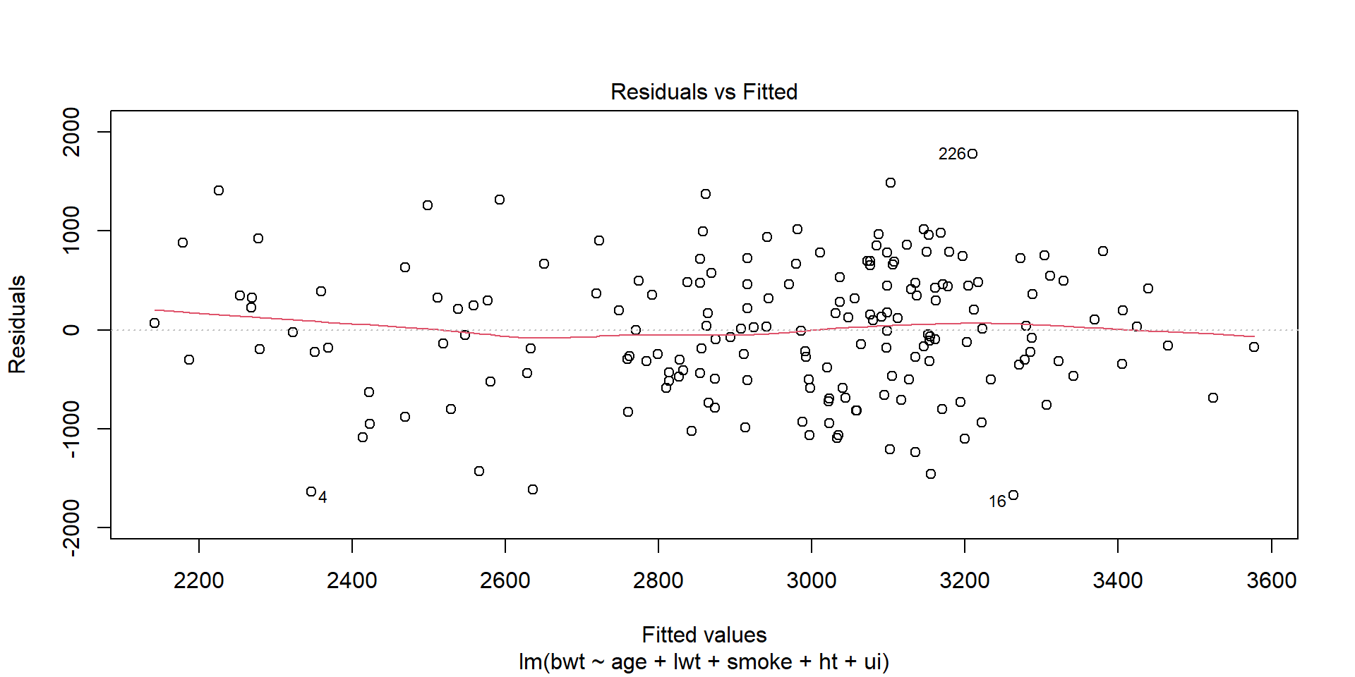
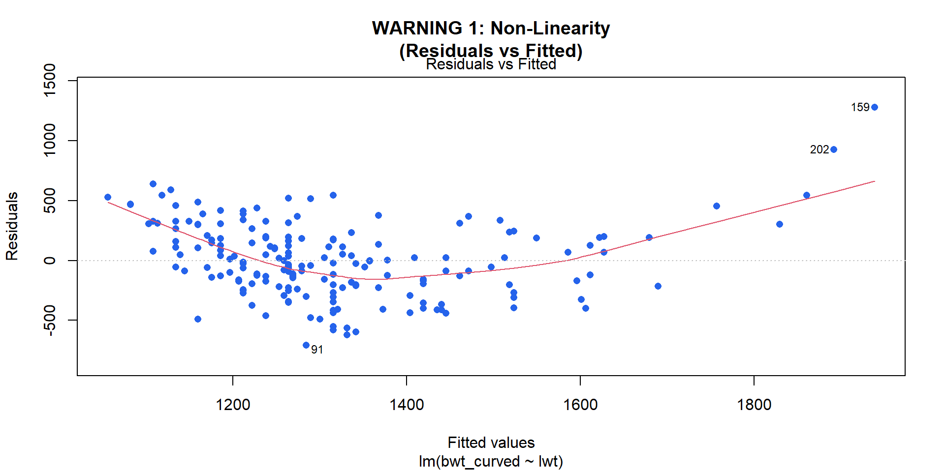
- Healthy Pattern: Residuals bounce randomly across a horizontal band centered at \(y = 0\), with no distinct trend. The red smooth smoother curve is nearly flat along \(y = 0\).
- Violation Warning: Distinct parabolic “U-shape”, inverted “U”, or sinusoidal wave.
I — Independence of Errors
Knowing that Patient A has an unexpectedly high outcome provides zero information about Patient B’s outcome.
Example
- Clustering: Patients recruited from the same hospital ward or family share correlated responses.
- Autocorrelation: Longitudinal measurements taken repeatedly over time on the same subject.
Actions
- Revise study design
- Clustered data: Linear Mixed-Effects Models (
lme4::lmer()) incorporating random intercepts for clusters/centers. - Tool: Evaluation of study design, Residuals vs. Time/Subject ID order
N — Normality of Residuals
- The error terms are normally distributed around the fitted line.
Crucial Clarification: In regression, the raw variables \(Y\) and \(X\) do not need to be normally distributed; only the residuals (\(\varepsilon_i\)) must be normally distributed.
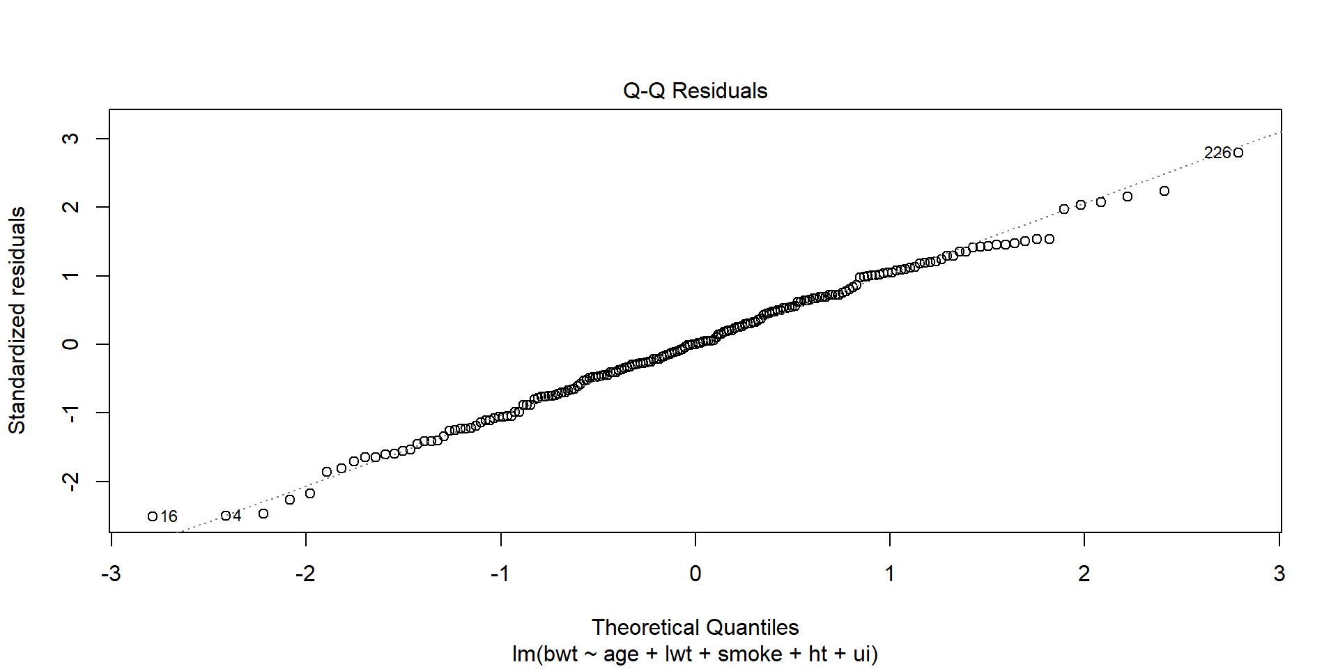
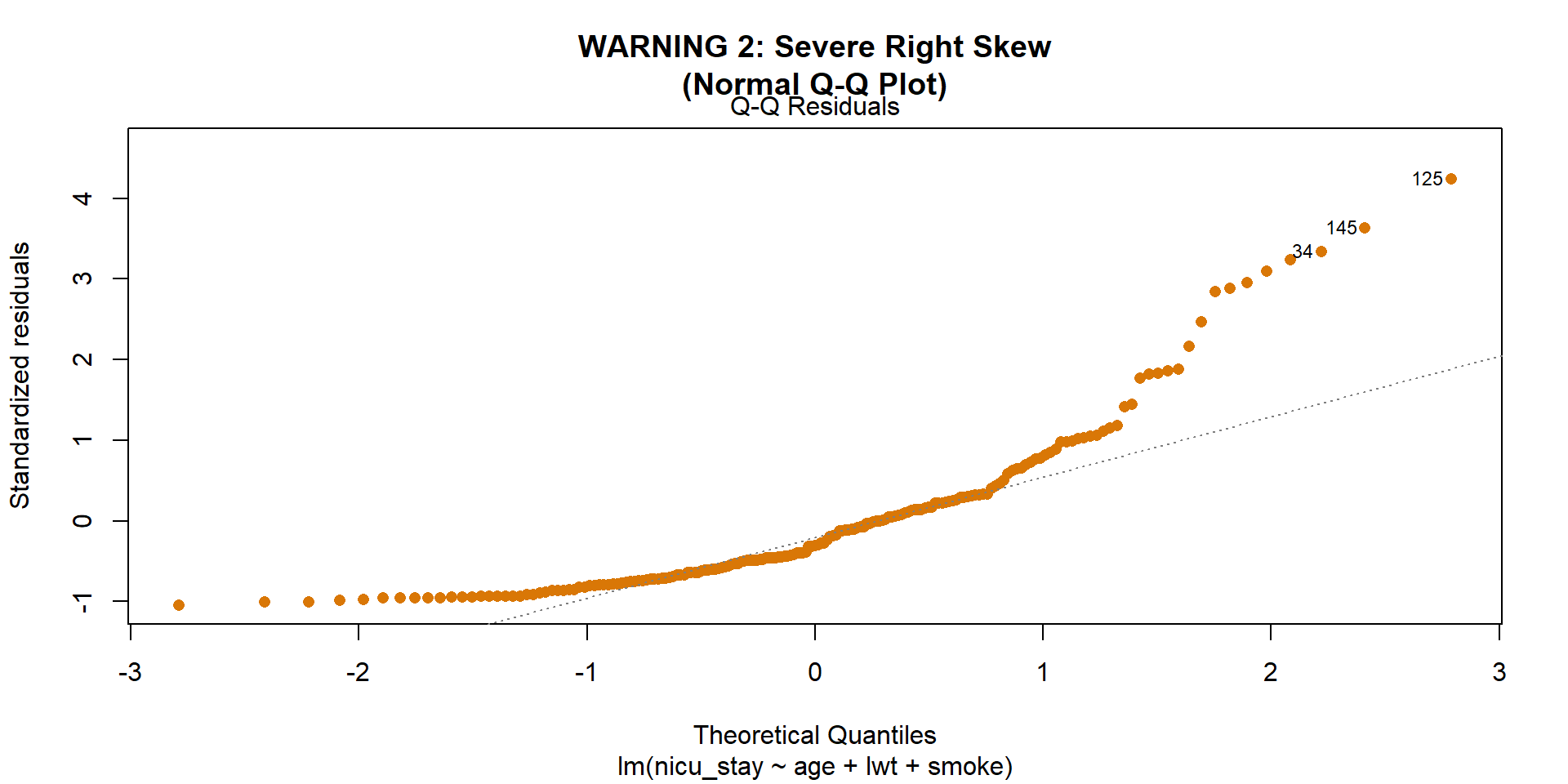
- Tool: Normal Q-Q Plot (Base R Plot 2:
plot(model, which = 2)). - Healthy Pattern: Residual quantiles fall tightly along the theoretical 45-degree dashed line.
Actions
- Transform the outcome variable: logarithmic transformation: \[\log(Y_i) = \beta_0 + \beta_1 X_i + \varepsilon_i\]
E — Equal Variance
- The variance of the residuals \(\text{Var}(\varepsilon_i \mid X) = \sigma^2\) is constant across all predicted values \(\hat{Y}\). (Homoscedasticity)
Consequence
- Conventional \(SE(\hat{\beta})\) calculations are invalid. If variance expands at higher values, standard errors are underestimated for higher exposures, leading to false claims of significance.
Actions
- Variance-stabilizing transformations: \(\log(Y)\) or \(\sqrt{Y}\).
- Heteroscedasticity-Consistent (HC) Robust Standard Errors: Using
sandwich::vcovHC(model, type = "HC3")paired withlmtest::coeftest(). - Weighted Least Squares (WLS): Weights inversely proportional to variance: \(w_i = 1/\sigma_i^2\).
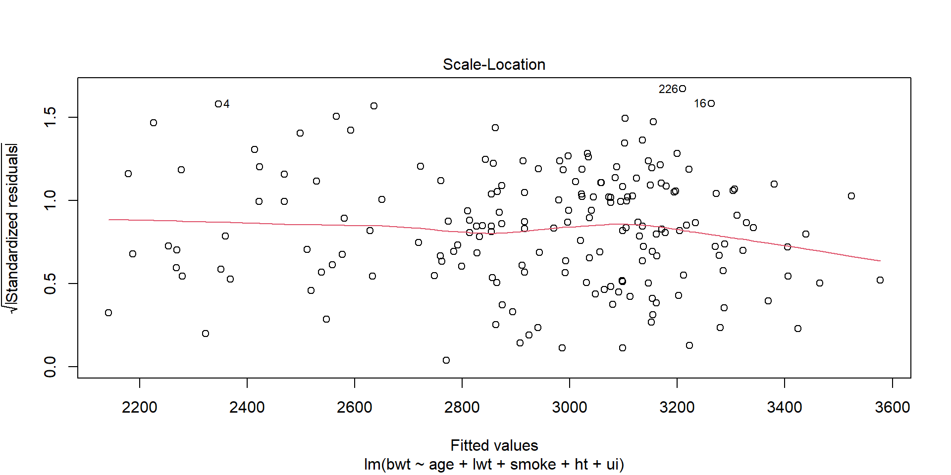
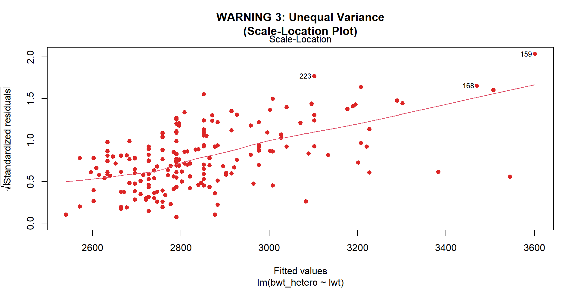
- Healthy Pattern: A horizontal smooth red line with an even, constant vertical scatter of points across all fitted values.
- Violation Warning: A megaphone / funnel shape where residual spread widens drastically as \(\hat{Y}\) increases (common in biomedical dosing and growth studies).
Summary Diagnostic Flowchart
                      [Fit Linear Model: lm(Y ~ X1 + X2)]
                                       │
                ┌──────────────────────┴──────────────────────┐
                ▼                                             ▼
       [Evaluate Goodness-of-Fit]                    [Validate L.I.N.E.]
       • R² & Adjusted R²                            • Residuals vs Fitted (Linearity)
       • Residual Std Error (RSE)                    • Study structure (Independence)
       • Global ANOVA F-Test                         • Normal Q-Q (Normality)
                │                                    • Scale-Location (Equal Variance)
                │                                             │
                └──────────────────────┬──────────────────────┘
                                       │
                     All L.I.N.E. Assumptions Hold?
                                       │
                      ├─── YES ──► Report slopes, 95% CIs & p-values
                      │
                      └─── NO  ──► Apply Diagnostic Remedy:
                                   • Non-linear? ──► Log(X), Polynomials
                                   • Heteroscedastic? ──► Log(Y), HC3 Robust SE
                                   • Non-normal? ──► Transform Y, Bootstrap
                                   • Clustered? ──► Mixed-Effects Model (lmer)
Eakins, Thomas. 1875. The Clinic of Dr. Gross. Oil on canvas. Philadelphia Museum of Art.